While the original post on Oracle has been removed, which limits our understanding of the exact data collection methodology, the dataset appears to have been personally compiled by the contributor. Despite these limitations, our research indicates that this dataset has been explored in various academic and practical contexts, as evidenced by its usage in projects hosted on platforms like Databricks and GitHub, which can be found at Databricks Project and GitHub - Insurance Fraud Claims Detection, respectively. These explorations suggest its high potential for academic research and application.
We acknowledge that obtaining proprietary insurance information is difficult and therefore there are not many publicly available datasets. Despite the lack of detailed background on data collection, we believe that this dataset offers a valuable opportunity to apply our classroom knowledge to real-world data.
As for importing the data, we downloaded it from the GitHub repository and then imported it into our local environment for analysis. We will provide a detailed description of the dataset’s characteristics, including its format and dimensions, in the Description part.
2.1 Description
The data is in .csv format. There are 1,000 rows with 40 columns, however, the column “_c39” is all null so we will drop it before our analysis.
There are 38 attributes (features) in total in the data. They can be divided into five main categories, which are Personal and Policy Information, Location and Vehicle Information, Incident Details, Claim Information and Other Attributes:
Personal and Policy Information: It contains columns for customer characteristics such as months_as_customer, age, policy_number, policy_bind_date, policy_state, policy_csl (Combined Single Limit), policy_deductable, policy_annual_premium, and umbrella_limit.
Location and Vehicle Information: There are details about the insured_zip, incident_location, incident_hour_of_the_day, as well as information about the vehicle involved like auto_make, auto_model, and auto_year.
Incident Details: The dataset includes specific details about incidents such as incident_date, incident_type, collision_type, incident_severity, authorities_contacted, and whether a police_report_available.
Claim Information: This encompasses the total_claim_amount, injury_claim, property_claim, vehicle_claim, and whether the claim was reported as fraud (fraud_reported).
Other Attributes: Additional attributes include details about the insured like insured_sex, insured_education_level, insured_occupation, insured_hobbies, insured_relationship, as well as information about witnesses, bodily injuries, and other aspects related to the insurance claims.
Below is what our data looks like:
Code
data <-read.csv('insurance_claims.csv', na.strings =c("?", "NA"))head(data)
  months_as_customer age policy_number policy_bind_date policy_state policy_csl
1                328  48        521585       2014-10-17           OH    250/500
2                228  42        342868       2006-06-27           IN    250/500
3                134  29        687698       2000-09-06           OH    100/300
4                256  41        227811       1990-05-25           IL    250/500
5                228  44        367455       2014-06-06           IL   500/1000
6                256  39        104594       2006-10-12           OH    250/500
  policy_deductable policy_annual_premium umbrella_limit insured_zip
1              1000               1406.91              0      466132
2              2000               1197.22        5000000      468176
3              2000               1413.14        5000000      430632
4              2000               1415.74        6000000      608117
5              1000               1583.91        6000000      610706
6              1000               1351.10              0      478456
  insured_sex insured_education_level insured_occupation insured_hobbies
1        MALE                      MD       craft-repair        sleeping
2        MALE                      MD  machine-op-inspct         reading
3      FEMALE                     PhD              sales     board-games
4      FEMALE                     PhD       armed-forces     board-games
5        MALE               Associate              sales     board-games
6      FEMALE                     PhD       tech-support  bungie-jumping
  insured_relationship capital.gains capital.loss incident_date
1              husband         53300            0    2015-01-25
2       other-relative             0            0    2015-01-21
3            own-child         35100            0    2015-02-22
4            unmarried         48900       -62400    2015-01-10
5            unmarried         66000       -46000    2015-02-17
6            unmarried             0            0    2015-01-02
             incident_type  collision_type incident_severity
1 Single Vehicle Collision  Side Collision      Major Damage
2            Vehicle Theft            <NA>      Minor Damage
3  Multi-vehicle Collision  Rear Collision      Minor Damage
4 Single Vehicle Collision Front Collision      Major Damage
5            Vehicle Theft            <NA>      Minor Damage
6  Multi-vehicle Collision  Rear Collision      Major Damage
  authorities_contacted incident_state incident_city  incident_location
1                Police             SC      Columbus     9935 4th Drive
2                Police             VA     Riverwood       6608 MLK Hwy
3                Police             NY      Columbus  7121 Francis Lane
4                Police             OH     Arlington   6956 Maple Drive
5                  None             NY     Arlington       3041 3rd Ave
6                  Fire             SC     Arlington 8973 Washington St
  incident_hour_of_the_day number_of_vehicles_involved property_damage
1                        5                           1             YES
2                        8                           1            <NA>
3                        7                           3              NO
4                        5                           1            <NA>
5                       20                           1              NO
6                       19                           3              NO
  bodily_injuries witnesses police_report_available total_claim_amount
1               1         2                     YES              71610
2               0         0                    <NA>               5070
3               2         3                      NO              34650
4               1         2                      NO              63400
5               0         1                      NO               6500
6               0         2                      NO              64100
  injury_claim property_claim vehicle_claim auto_make auto_model auto_year
1         6510          13020         52080      Saab        92x      2004
2          780            780          3510  Mercedes       E400      2007
3         7700           3850         23100     Dodge        RAM      2007
4         6340           6340         50720 Chevrolet      Tahoe      2014
5         1300            650          4550    Accura        RSX      2009
6         6410           6410         51280      Saab         95      2003
  fraud_reported X_c39
1              Y    NA
2              Y    NA
3              N    NA
4              Y    NA
5              N    NA
6              Y    NA
2.2 Research plan
Our project will initially focus on an exploratory analysis of each category of data in the dataset, aiming to unearth potential connections among them and their relationship with insurance fraud. Then we will employ techniques such as regression analysis and Principal Component Analysis (PCA). These methods will enable us to compare and quantify the impact of different factors on the likelihood of fraud.
By conducting this multi-dimensional analysis, we will leverage the dataset’s comprehensive range of data - encompassing geographical trends, policy features, demographic characteristics, incident specifics, and vehicle information. This approach will not only help us identify patterns and insights in each data category but also allow us to understand the cumulative impact of these factors on insurance fraud.
2.3 Missing value analysis
In this dataset, all the missing data are represented by “?” elements, so we need to replace all “?” elements with null values. Besides, there is one column named “_c39” with all null values that can be dropped.
Code
data <-read.csv('insurance_claims.csv', na.strings =c("?", "NA"))data <-subset(data, select =-X_c39)
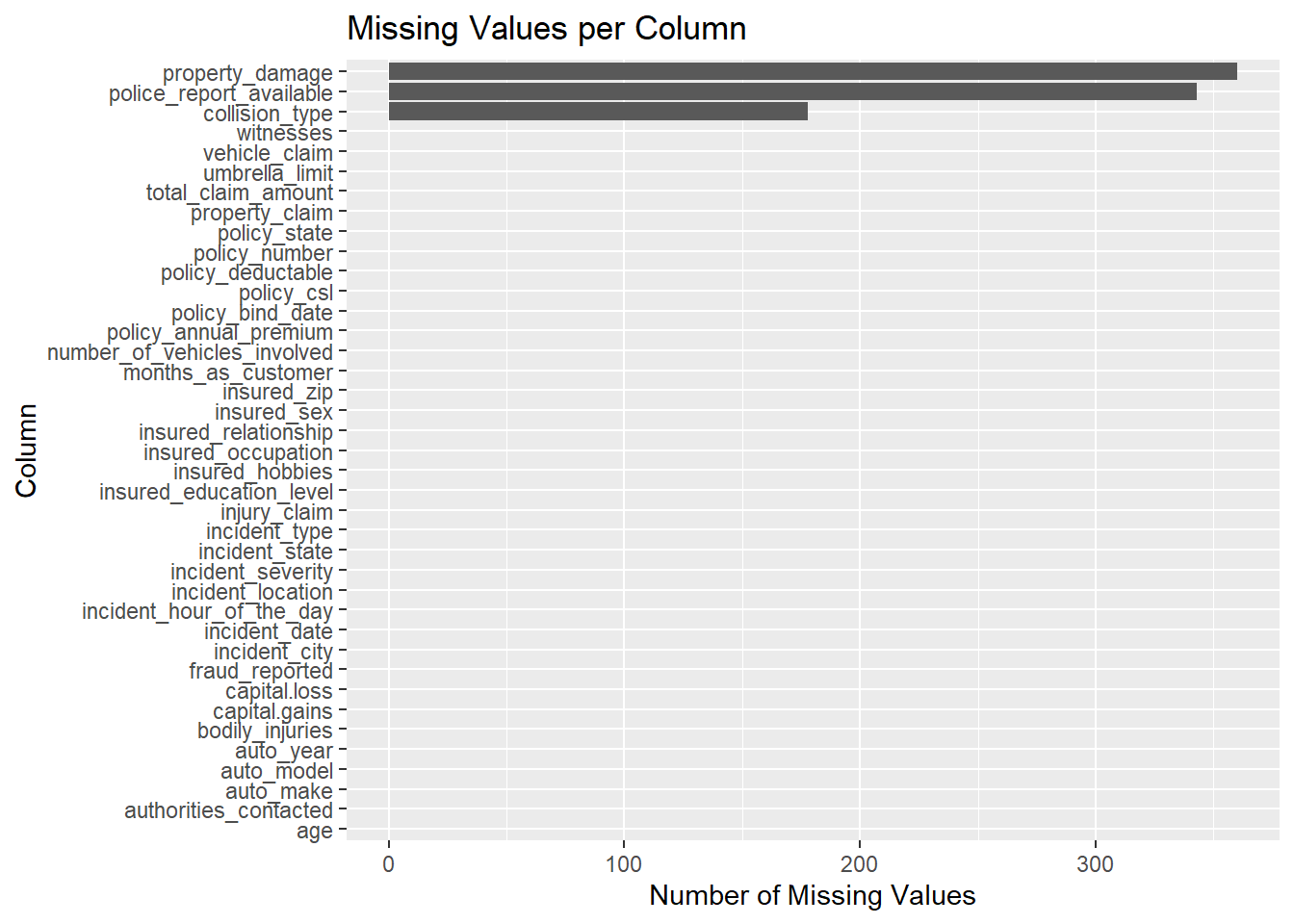
Then calculate the number of missing values in each column and visualize the missing data using a bar plot for an overview.
Code
library(ggplot2)library(dplyr)# Count missing valuesmissing_values <-sapply(data, function(x) sum(is.na(x)))missing_data_frame <-data.frame(column =names(missing_values), missing_count = missing_values)# Create a data frame for plottingmissing_data_frame <-data.frame(column =names(missing_values), missing_count = missing_values)# Create the bar plot with ggplot2ggplot(missing_data_frame |>arrange(desc(missing_count)), aes(x =reorder(column, missing_count), y = missing_count)) +geom_bar(stat ="identity") +coord_flip() +# Reverse the coordinate systemxlab("Column") +ylab("Number of Missing Values") +ggtitle("Missing Values per Column") # Add titles and labels as needed
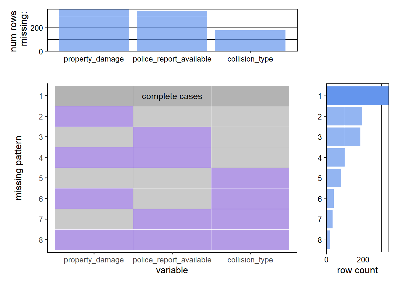
Obviously, there are only three columns with missing values, so we proceed to drop all the other columns and use plot_missing in redav to plot the them.
The patterns indicated by these plots suggest that the missing data is mostly concentrated in a single variable which is illstrated by the fact that case 2 and 3 in missing pattern are significantly more than other cases. Missingness spreading across several variables needs to be handled carefully, as it could bias the results of any analysis performed on the dataset. Techniques such as imputation or the use of models that can handle missing data might be necessary to account for the missing values.